
Recognizing digits using dynamic time warping
In this post I’ll write about my attempt at the digit recognition Kaggle competition. The goal is to accurately recognize single hand-written digits, which are provided as two-dimensional grayscale images. Each pixel element is an integer value in the range [0, 255].
Here’s what a typical digit from the dataset looks like:
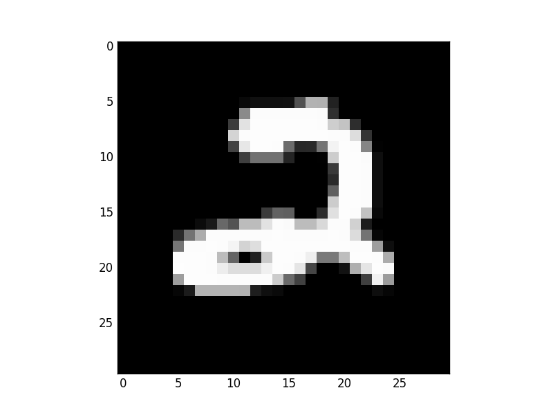
To solve the challenge, I used an algorithm called dynamic time warping (DTW). It’s a nifty little method that provides an intuitive way of comparing different signals (in this case, the digits). In this post, I’ll do my best to explain how the method works and how successful my implementation of it was in recognizing digits.
Dynamic time warping
Dynamic time warping is an algorithm used to quantify how similar two signals are. The method is usually used to compare time-series data, and in fact, was developed in the 70’s primarily for the purpose of speech recognition. The data doesn’t have to be a time-series, though; actually, all that is required is that we are able to represent our data in some way as x-y data. For brevity and for historical reasons, I’ll refer to the x-y representation of the data as a time series, even though it is not what we would traditionally view as a time-series.
Representing the digits as time-series data
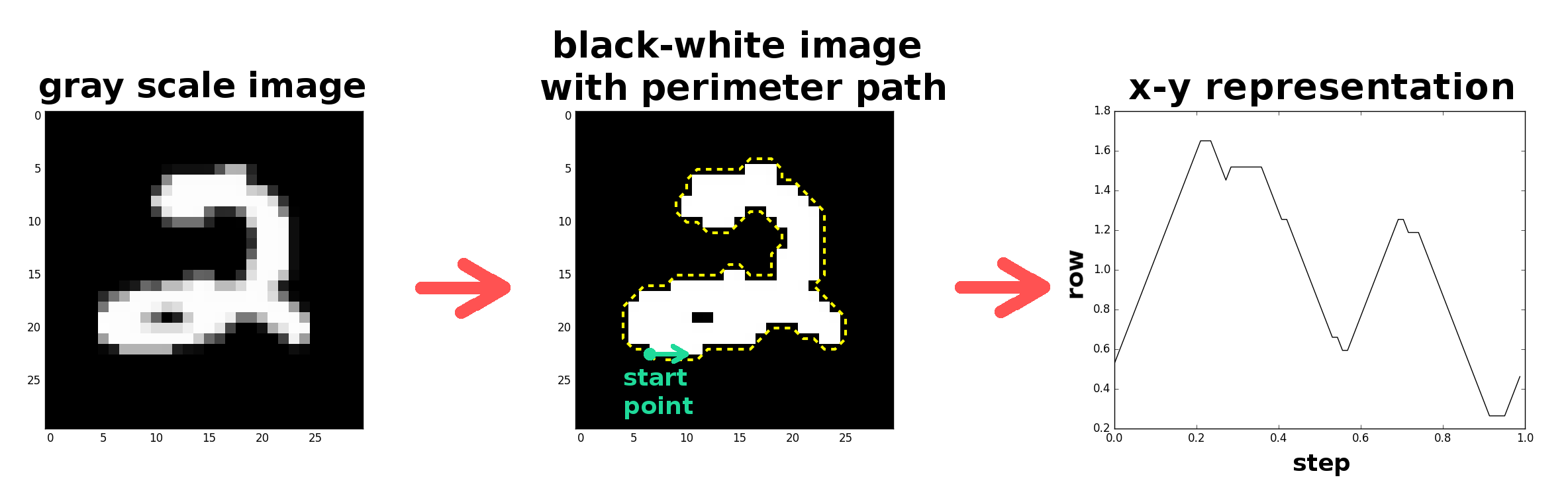
Right now you may be scratching your head–how do we get a time-series out of our data type, a grayscale image with pixel values? There are any number of ways one could think about transforming the data, but this is how I did it. First, I converted the grayscale representation of each character to a black/white representation; the digits are still identifiable as black and white images and it drastically simplifies the identification task. To create a time-series of the black and white image, I “walked” around the digit’s perimeter, recording at each step in the walk the row and column designating our position. This process actually produces two time-series. The time-axis corresponds to the step number in the walk, and the y-axis corresponds to either the row or column position at that step.
As an aside, the cool thing about DTW is how adaptable it is to different problems. As long as we can come up with some method of representing our data in the form of a time-series, we can apply DTW.
Here’s what the representation change looks like:
Now that we have the representation transformation down, we need to quantitatively calculate the ‘difference’ between different characters’ time series.
Comparing the digits
The simplest way to quantify the difference between two time-series is via a simple time-aligned Euclidean distance metric. Simply put, we take the two time-series, align them on the time-axis, and sum the distance between every pair of aligned points in the data set.
The more similar the two time series are, the lower this cumulative difference is. Here’s a visualization of the time-aligned Euclidean distance metric (a small y-displacement was added to one of the signals for the sake of visualization):
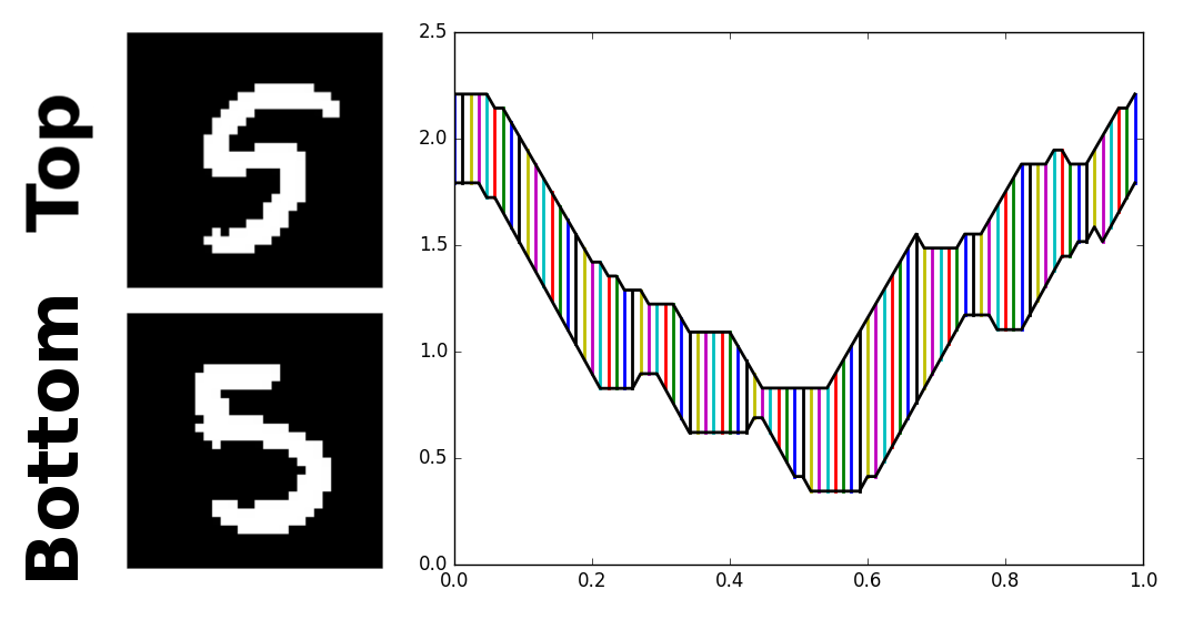
Looking at the time-series representations of the two fives, we can see that they are similar, but not quite aligned in the time-axis. For example, a much better fit could be achieved if only we were allowed to just slightly shift and stretch the bottom most data points in the lower time-series to the left. In effect, our eyes can see what the distance metric does not–that the two signals are more similar than they are given credit for.
This is where DTW comes in–DTW is an algorithm that allows for a non-linear ‘warping’ of the time axis so as to minimize the cumulative distance between two time series. It also has the advantage that the time-series do not need to have the same number of data points.
We start with DTW by constructing a matrix of the distance between all pairs of data points between the two time series.
Here’s what the distance-matrix looks like for the two fives from above:
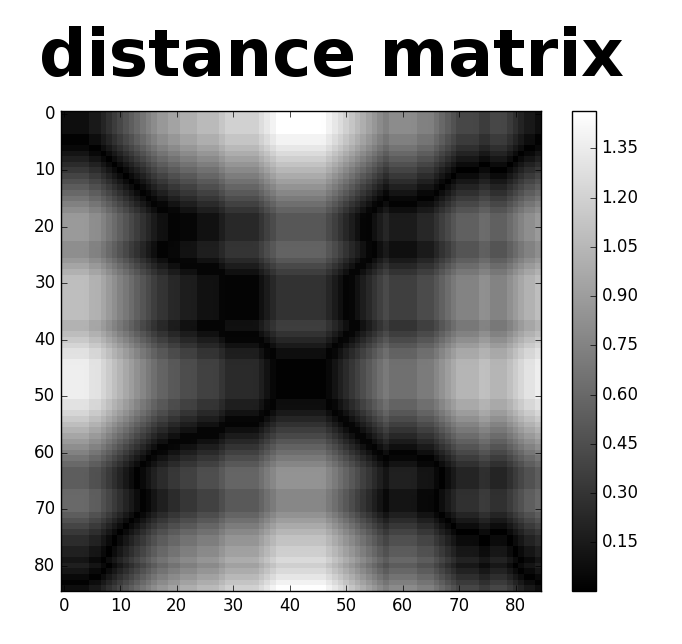
Our goal is to find a path through this matrix that has the lowest cumulative distance; this path corresponds to the time warping that gives the best match between the two time series. The cumulative distance along any particular path is called the cost of that path.
There are a few requirements that the minimal cost path must satisfy. They are:
- The beginning and end points of both series must match up. This means the past must path through the upper-left and lower-right corners of the above matrix. If the two time-series have m and n data points respectively, the path must pass through the points (0, 0) and (m-1, n-1).
- The path must progressively step through the matrix one row, one column, or one row and one column at a time, i.e., if (i, j) is a point along the path, the next step must be any of (i+1, j), (i, j+1), or (i+1, j+1).
- Optional constraints: -If we don’t want to allow any extreme warping to happen (i.e., large time distance between matched data points) we can impose restrictions on where the warping path is allowed to go in the matrix. -A constraint on the maximum number of points a single point can be connected to. This corresponds to limitations on the maximum and minimum values the slope in the path can have.
We now know the purpose of the time warping and the requirements that the minimum cost path must satisfy, so how do we actually find that minimum path? As the name of the algorithm suggests, we solve for the minimum cost path dynamically. The key is this: the minimum cost path between points (0, 0) and (i, j) must pass through (i-1, j), (i-1, j-1), or (i, j-1) (property 2 above). This means we can iteratively calculate the minimum cost to get to (m-1, n-1) by starting at (0, 0) and calculating the minimum costs for paths starting at (0, 0) and ending at (1, 0), (0, 1), (1, 1), (2, 1), …, (m-1, n-1). Note that this does not yield the path itself (we can calculate that after), but it does give us the cost of the optimal warping.
Here’s some Python style pseudo-code for calculating the cost of the minimum cost path to (m-1, n-1):
def distance(a, b):
  return abs(a-b)

cost_matrix = numpy.zeros((m, n))
cost_matrix[0, 0] = abs(y1[0] - y2[0])
for i in range(m):
  for j in range(n):
    if i == 0: #Top row; edge positions must be treated separately
	  cost_matrix[i, j] = distance(y1[i], y2[j]) + cost_matrix[i, j-1]
	elif j == 0: #Left column
	  cost_matrix[i, j] = distance(y1[i], y2[j] + cost_matrix[i-1, j])
	else:
	  cost_matrix[i, j] = distance(y1[i], y2[j]) +\
	  minimum(cost_matrix[i-1, j], cost_matrix[i-1, j-1], cost_matrix[i, j-1])
The measure of how well the two signals match is then given by cost_matrix[m-1, n-1].
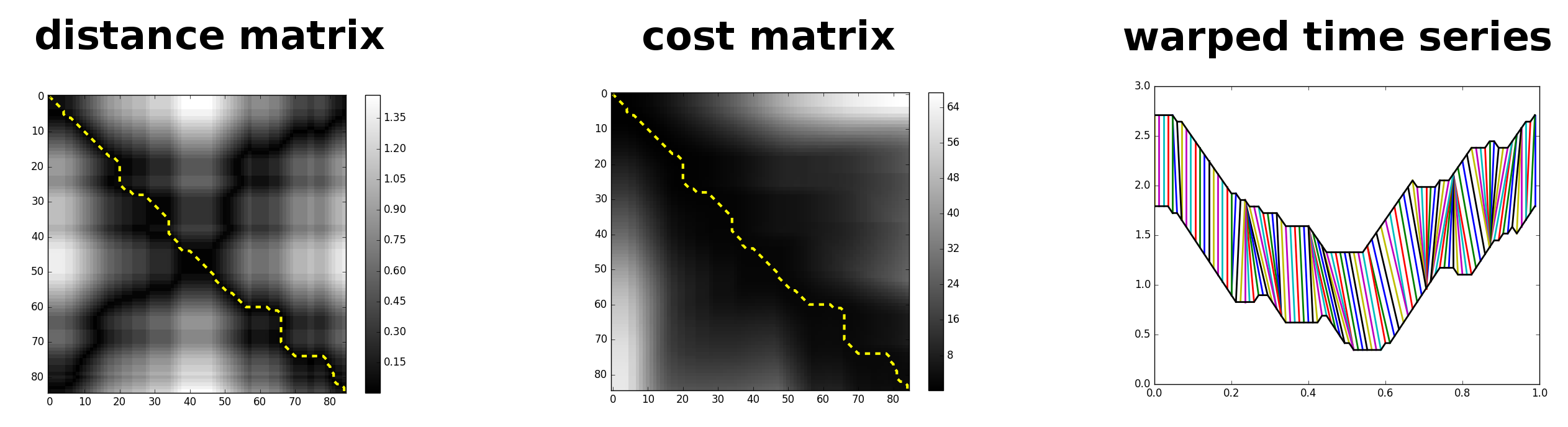
Finally, it can be useful to visualize the warping by looking at what the path actually looks like. The optimal warping path itself is found by starting at the end point (m-1, n-1) and ‘walking’ to (0,0), at each step walking to the adjacent matrix element with the lowest minimum cost. Below we have the distance matrix, cost matrix, and plots of the two time-series showing the warping that the algorithm has provided. Note the difference between the non-warping (above) and warping plots.
Results
The above algorithm described how to calculate the difference between two digits. The kaggle competition asked for us to classify unknown digits from a test set. To do this, I calculated the cost value between a given test digit and a set of k training samples for each digit. The test digit is then classified by the k training samples with the lowest total cost (the best overall fit between all training examples).
Here are the results of the algorithm:
| Test | Correct | Total | Ratio | |||
|---|---|---|---|---|---|---|
| digit | predictions | predictions | ||||
| 0 | 815 | 1090 | 0.75 | |||
| 1 | 1151 | 1249 | 0.92 | |||
| 2 | 702 | 1102 | 0.64 | |||
| 3 | 1018 | 1106 | 0.92 | |||
| 4 | 958 | 1093 | 0.88 | |||
| 5 | 740 | 971 | 0.76 | |||
| 6 | 891 | 1058 | 0.84 | |||
| 7 | 1083 | 1177 | 0.92 | |||
| 8 | 716 | 1054 | 0.68 | |||
| 9 | 784 | 1100 | 0.71 | |||
| Total | 8858 | 11000 | 0.81 |
The data shows that the method is just ok getting roughly four of every five classifications correct. All in all I think this is ok for a method that was not developed to handle this type of problem at all. Another point to make is that there are a number of different varieties of DTW that exist that potentially could be used to improve the digit recognition record. Two flavors of DTW I’ll point out are derivative dynamic time warping (DDTW) and weighted dynamic time warping (WDTW). As the name implies, in DDTW the distance between two points is given by the difference in their local derivatives, not their amplitudes. This method is especially useful if we have features that differ in amplitude but have similar shapes. For example, the method would more properly match two peaks that differ in amplitude. WDTW works by adding a factor to the distance between two points based on their time separation. Points that are closer together in time between the two signals are given greater weights than points further apart; the effect of the weight addition is to add a sort of stiffness to the warping procedure.
If you’re interested in learning more about DTW, I suggest visiting Prof. Keough’s page, who has done a lot of work on the method. In particular, I found this paper helpful.
comments powered by Disqus