I recently started working on a project where the goal is to find periodicity within a time series. The naive solution is pretty straight forward: look for peaks in the series’ power spectral density. However the naive approach doesn’t work for my data set, and I suspect it won’t work for many other applications as well. Two reasons why:

1. The data is not regularly sampled.

The data set I’m working with is gamma ray counts from the Fermi space telescope. Because Fermi is in orbit around the Earth, it can’t stay pointed at the same object continuously. Instead, it takes a rapid series of measurements while it is on the same side of the Earth as the star until the star again goes out of view. The resulting distribution of exposures that Fermi takes looks like this:

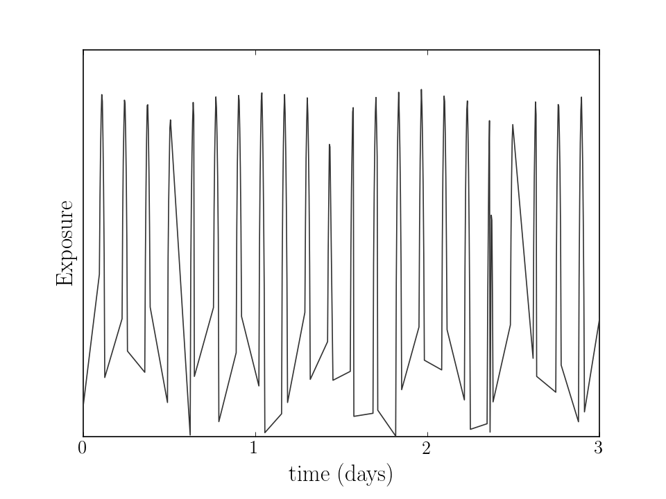
It’s clear that the exposures and hence the resulting time-series are not evenly sampled, but how does that effect the power spectrum? Remember that the power spectrum is the squared modulus of the (discrete) Fourier transform of the time-series. Calculation of the dFT requires that the data be evenly sampled, which isn’t the case for the Fermi data. We could down sample the data, taking one data point every orbital period and calculating the PSD of the downsampled time-series, but that would be discarding a serious amount of data which is seldom practical.

2. The periodic part of the signal is faint.

I won’t go into the astrophysics here of where the periodicity in our Fermi data comes from, but the effect is subtle. A straight-forward calculation of the power spectral density doesn’t yield enough accuracy for us to find a peak.

Fortunately, problems 1 and 2 already have solutions. Whenever data is irregularly sampled as our Fermi data is, we can calculate something similar to the PSD called the Lomb-Scargle periodogram. The L-S periodogram has the same interpretation as the PSD, but uses a different formula. To tackle the issue of faint signals, there’s something called Welch’s method that can be used to smooth noisy PSDs. The objective of this blog post is to apply Welch’s method to calculate Lomb-Scargle periodograms. Along the way, I’ll talk about the general idea of the PSD and Welch’s method, applied to an artificial time-series consisting of a periodic signal over a noisy background. All of the analysis will be performed in Jupyter notebooks running Python 2.7 code.

Quick aside before jumping in: what we’re actually calculating here is the periodogram of the signal–not the power spectrum. IMO this is a technical distinction; the power spectrum and periodogram differ only in that one is calculated via the Fourier transform of an infinite, continuous signal and the other via the discrete Fourier transform of a finite, discrete signal. In spirit the two calculate the same thing, namely the frequency dependence of the signal intensity, and you’ll more often than not hear people refer to the periodogram as the ‘spectrum’, ‘power spectrum’, or ‘power spectral density’ (these terms are often used interchangably).

Welch’s method for an evenly sampled data set

Generating the signal

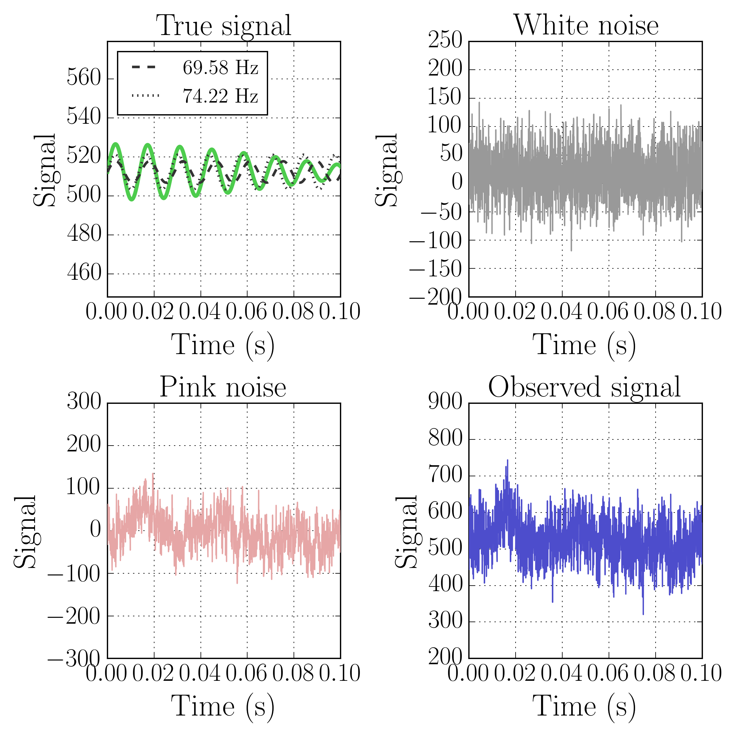
Consider a time-series of measured data that is the superposition of the signal-of-interest and noise. To make things interesting, let’s say that the underlying physical process that generates the signal has two fundamental frequencies and that the noise is a superposition of white noise and pink, or $\left(1/f\right)$, noise.

Here’s the Python code to generate the signal and noise:

The signal is generated by adding two sin functions of different frequencies. White-noise, which is a random signal with no time-correlation, is sampled from a normal distribution. To generate the pink noise, I took the inverse Fourier transform of the square root of the \(1/f\) power spectrum, giving each frequency component a uniformly distributed random phase.

And here are plots of the signal, both noise terms, and the total measured time-series:

Calculating the periodogram

Now we’ll compute the periodogram of the signal, which has the formula

$$S\left(f\right)=\left\lvert \hat{x}\left(f\right)\right\rvert^{2}=\frac{\Delta t}{N}\left\lvert\sum_{n=0}^{N-1}x_{n}e^{-i2\pi n\Delta tf}\right\rvert^{2},$$

where \(x\) is the measured signal, \(N\) is the number of samples, and \(\Delta t\) is the sampling rate.

We could calculate the periodogram ourselves using the above formula for the dFT, but I’ll just go ahead and directly compute it using the periodogram function from the scipy.signal package.

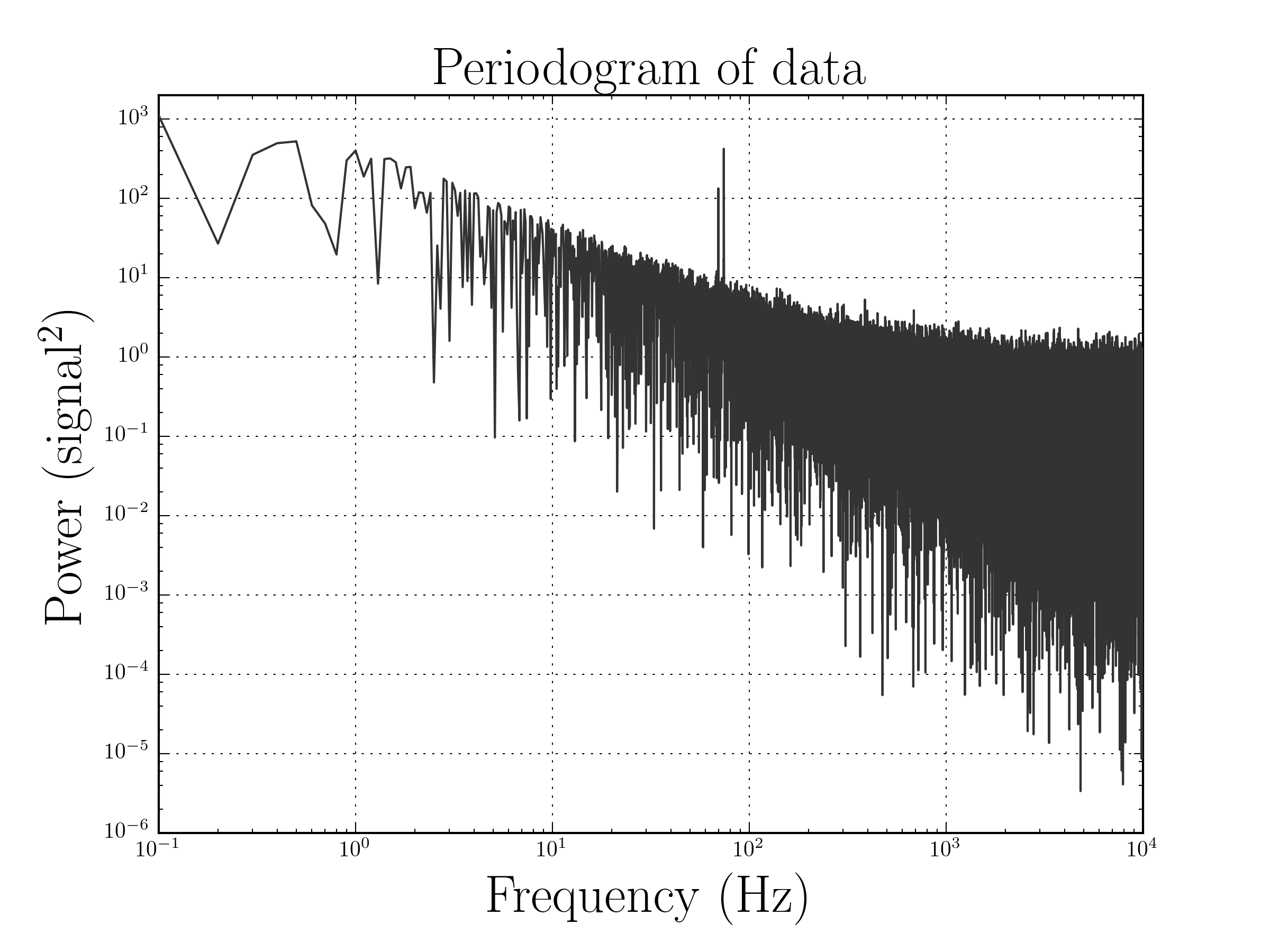
As you can see in the PSD, there are two distinct peaks at the two frequencies from our signal. Cool, huh? It’s pretty remarkable that the method can be used to find periodicity when it’s completely unrecognizable in the observed signal.

Welch’s method

Even though the periodogram does reveal the two frequencies in the signal, it’s often desirable to smooth the periodogram. For this we employ Welch’s method, which basically just calculates the periodograms of segments of the signal and averages them.

Here’s the process in detail:

1. Break the time-series into \(M\) segments of length \(N_{m}\), which have overlap \(\alpha\).

2. Multiply the segment by a window-function, an amplitude modulating function.

3. Calculate the periodogram for each windowed-segment.

4. Average the periodograms.

For the following analysis, I used a Hanning window defined by the function \(w\left(n\right) = 0.5\left(1-\text{cos}\left(\frac{2\pi n}{N_{m}-1}\right)\right)\)

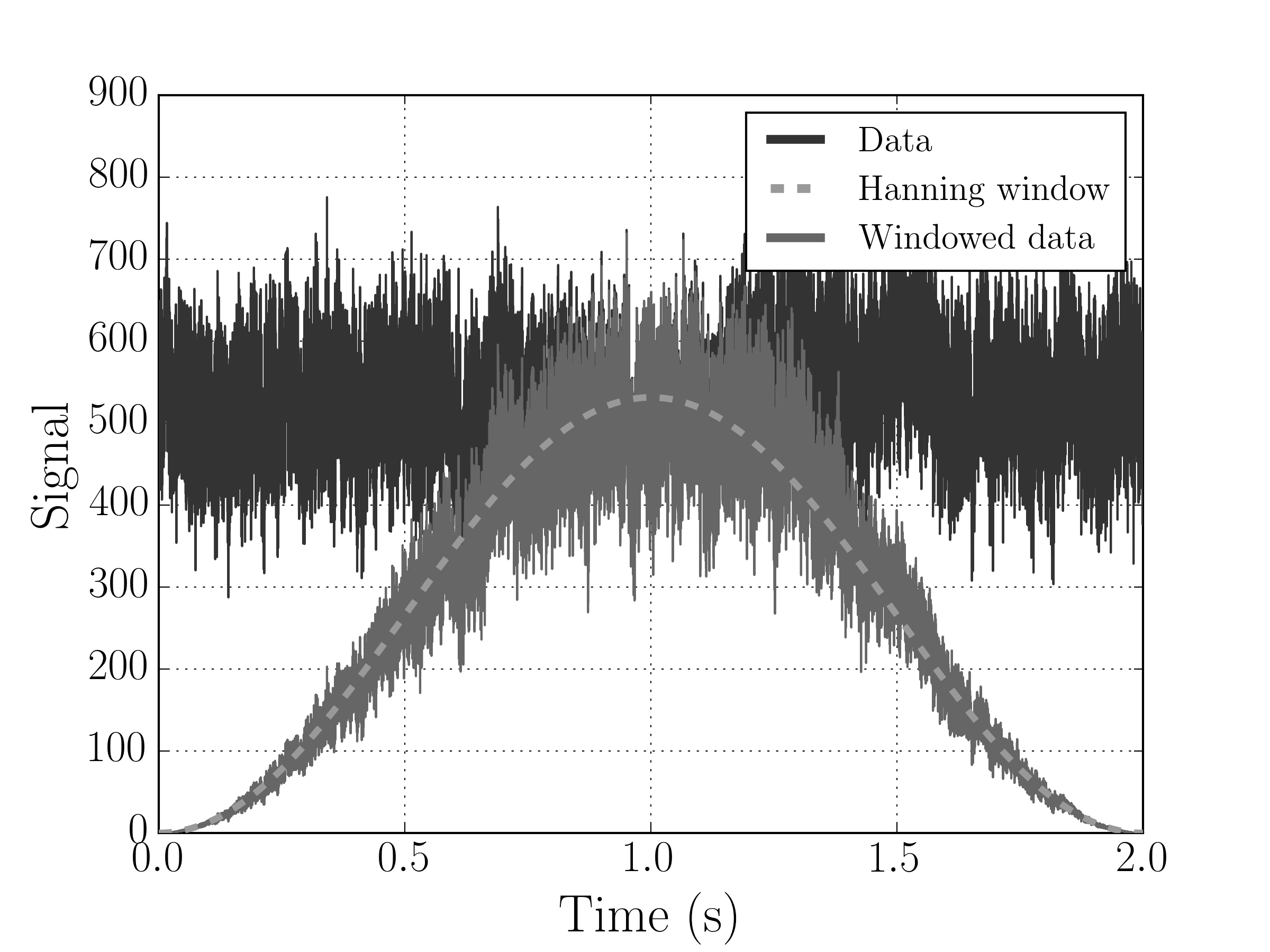
After windowing the data, calculating and averaging all of the periodograms, the spectrum looks like this:

That’s quite an improvement! However, one thing to point out is that we lose some information about the low-frequency power of our signal by windowing the data. But, if we’re confident that the periodic processes in our signal are much faster than the windowing interval (and hence our total measurement interval), then windowing the data and applying Welch’s method doesn’t result in the loss of much information.

Welch’s method for a an unevenly sampled data set

Now, let’s perform the same analysis but for data that is not uniformly sampled. To do this, I’ll take the same time-series from the previous example but randomly remove 75% of the data points. Here’s what the new reduced data set looks like:

Calculating the Lomb-Scargle periodogram

Just as with the periodogram, I’ll use a Python package to calculate the L-S periodogram. The implementation I’m using comes from the AstroPy package written by Jake Vander Plas. Now, here’s the L-S periodogram calculated for the reduced data:

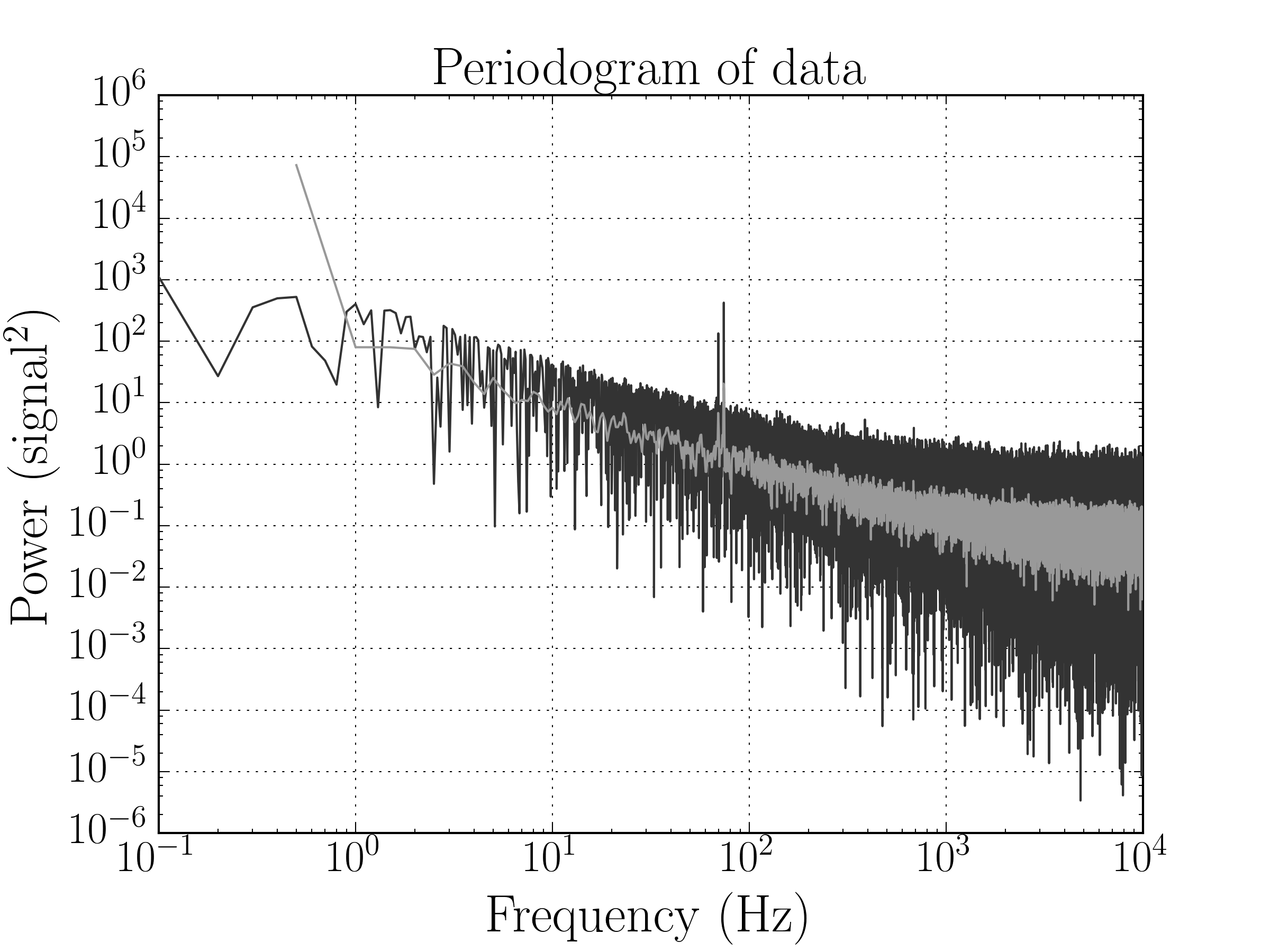
Applying Welch’s method

Finally, let’s apply Welch’s method to the reduced data. This is actually a little bit tricky, since it’s not entirely clear how the windowing should be done for non-uniformly sampled data. There are two options:

1. Window the data over a fixed number of data points.
2. Window the data over a fixed time.

comments powered by Disqus