This is the first entry in a multi-part introductory series on nanopores.

Nanopore?

The most precise definition of nanopore: a hole with opening diameter on the order of 1 nm in size. I’ll be the first to admit that this definition is a little dry, but there are a number of reasons, both academic and practical, that make nanopores worth studying. Nanopores exist naturally in nature, where they can be found in cells’ membranes and act as channels that enable transport of water molecules, ions, and biomolecules. Many natural nanopores have interesting transport properties; for example, potassium ions diffuse freely through a potassium channel while sodium ions are blocked, despite the two ions being nearly identical in size and charge.

It is also possible to fabricate synthetic nanopores. One distinct advantage of synthetic pores is the ability to tailor their geometry to the application at hand; on the other hand, biological pores have a fixed size and shape. There are a number of different applications for both types of nanopores, including ionic circuitry, water desalination, DNA sequencing, and biomolecule detection. Going back to the basic definition of nanopores ‘a 1 nm in diameter hole’, it is not immediately apparent why they are able to perform in all these applications. It turns out that the reason for their non-trivial transport properties is in something called the electrical double layer, or EDL. In the rest of this blog post we’ll look into the EDL, and in the rest of the posts we’ll explore how it affects transport in nanopores.

The electrical double layer

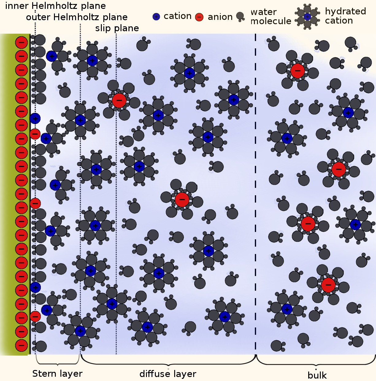
In the bulk, a symmetric ion solution is composed of equal parts cation and anion and the total solution charge is neutral. As we approach a charged surface, the electric potential from the surface makes it more energetically favorable for ions of the opposite polarity–counterions–to populate the solution compared to coions. This region of net charge in the solution, approximately within ~1 nm of the surface, is known as the diffuse layer. Right at the surface there is a thin layer of adsorbed ions and partially bound ions and water molecules called the Stern layer. Together, the Stern and diffuse layers make up the electrical double layer, or EDL. Sometimes the terms electrical double layer and diffuse layer are used interchangably; in the rest of this post we’ll discuss the diffuse layer but continue using the term EDL. Below is a cartoon of the structure of the solution near a negatively charged surface.

EDLs typically range from ~0.1-10 nm in thickness. Suppose we have a charged cylindrical nanopore of variable radius; the following plot shows the fractional volume of the EDL compared to the bulk, for an EDL length of 1 nm.

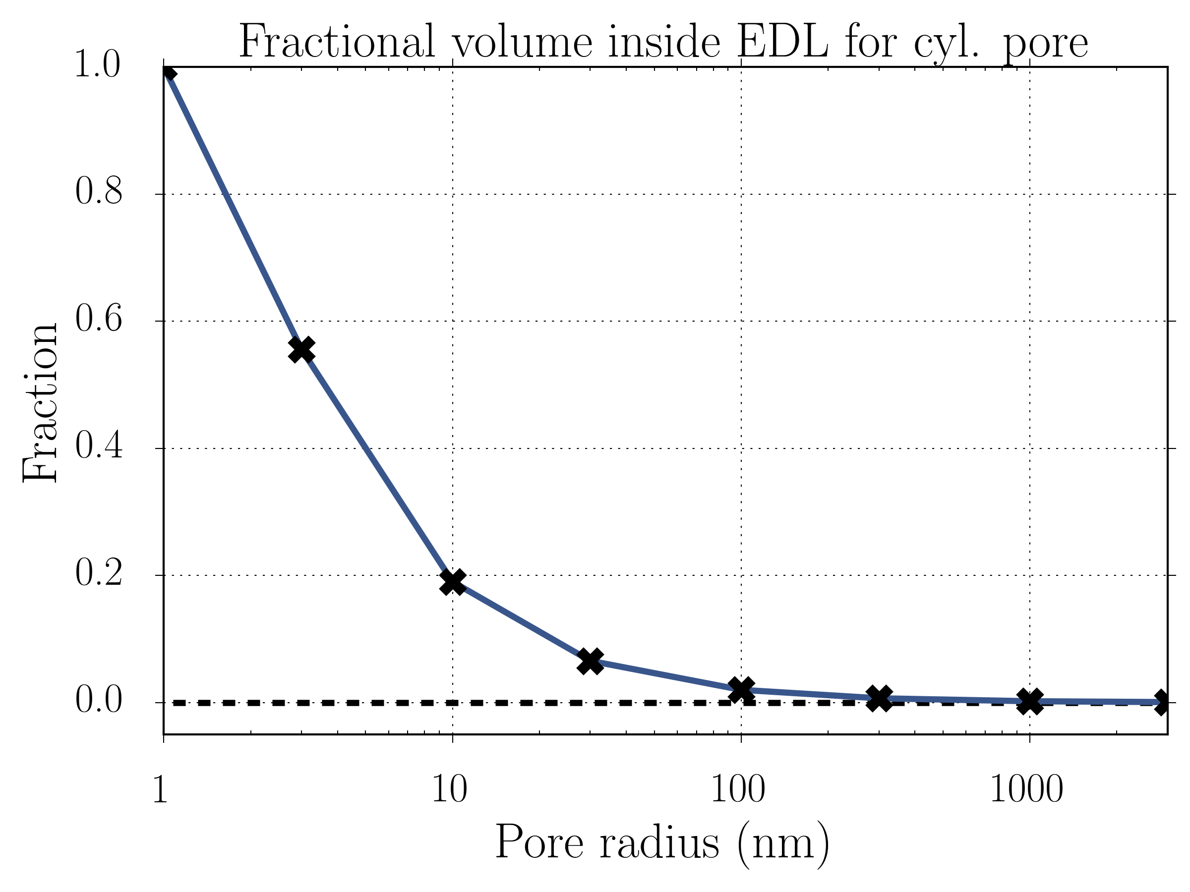
Notice that at around 100 nm the fraction of the ion solution within the EDL becomes appreciable and rapidly increases as the pore shrinks further into the nanoscale. For this reason, even though we typically define nanopores as holes around 1 nm in size, nanopore-like behavior can exist for pores having diameters of tens of nanometers.

Derivation

We can understand the formation of the electrical double layer as a competition between diffusion (chemical potential) and electrostatic forces (electric potential).

Consider an infinite planar surface with constant surface charge $\sigma$, and a solution composed of water and two types of oppositely charged ions with the same valency $z$ dissolved in the solution with bulk number density $C_{0}$. We seek to find the number density of each ion species $C^{+}$ and $C^{-}$ in the solution. The relevant equations here are Poisson’s equation, which relates the electrostatic potential to the charge distribution, and the Boltzmann distribution, which yields the probability distribution for particles to occupy an energy range.

$$\begin{equation} \tag{Poisson's equation} \nabla^{2}\psi=-\rho/\epsilon_{r}\epsilon_{0}=-ze\left(C^{+}-C^{-}\right)/\epsilon_{r}\epsilon_{0} \end{equation}$$ $$\begin{equation} \tag{Boltzmann distribution} C^{\pm}=C_{0}e^{E^{\pm}/k_{B}T}=C_{0}e^{\mp ze\psi/k_{B}T} \end{equation}$$

In the above equations, $\psi$ is the electrostatic potential arising from the free ions and the surface charge, and $\rho$ is the net charge density at a given position. Note that because the boundary in our system is an infinite plane, we can reduce Poisson’s equation to one-dimension, replacing the Laplace operator with a second derivative in one direction only. We’ll call it the $x-$direction. We combine the equations by inserting $C^{\pm}$ from the Boltzmann equation into Poisson’s equation. Doing so, we arrive at the full Poisson-Boltzmann equation:

$$\begin{equation} \tag{Poisson-Boltzmann equation} \frac{d^2\psi}{dx^{2}}=\frac{2zeC_{0}}{\epsilon_{r}\epsilon_{0}}\text{sinh}\left(\frac{ze\psi}{k_{B}T}\right) \end{equation}$$

The two boundary conditions for the 2nd order differential equation are:

1. $\int_{0}^{\infty}\rho\left(x\right)\text{dx}=\sigma$ and
2. $\frac{d\psi}{dx}\vert_{x\rightarrow\infty}=0$,

which come from the requirements that the solution is neutral overall, and that there are no electric fields in the bulk, respectively. The non-linear Poisson-Boltzmann equation can be linearized and easily solved if $ze\psi/k_{B}T\ll1$, leading to the Debye-Hückel equation, a good approximation in many cases. However, there is still an analytic solution in the general case. Solving the Poisson-Boltzmann equation yields the following formula for the electrostatic potential $\psi\left(x\right)$, and hence, the ion number densities $C^{+}\left(x\right)$ and $C^{-}\left(x\right)$:

$\begin{equation} \tag{Electric potential} \psi^{*}=2\log\left(\frac{1+\tanh\left(z\psi^{*}_{0}/4\right)e^{-\kappa x}}{1-\tanh\left(z\psi^{*}_{0}/4\right)e^{-\kappa x}}\right) \end{equation}$,

where $\psi^{*}=ze\psi/k_{B}T$, and $\kappa=\sqrt{\frac{2z^{2}e^{2}C_{0}}{\epsilon_{r}\epsilon_{0}k_{B}T}}$. The electrostatic potential at the surface, $\psi_{0}$, is related to the surface charge density via the Grahame equation:

$$\begin{equation} \tag{Grahame equation} \sigma=\frac{\epsilon_{0}\epsilon_{r}\psi_{0}}{\lambda_{D}}\left[\frac{2}{z\psi^{*}_{0}}\sinh\left(\frac{z\psi^{*}_{0}}{2}\right)\right] \end{equation}$$

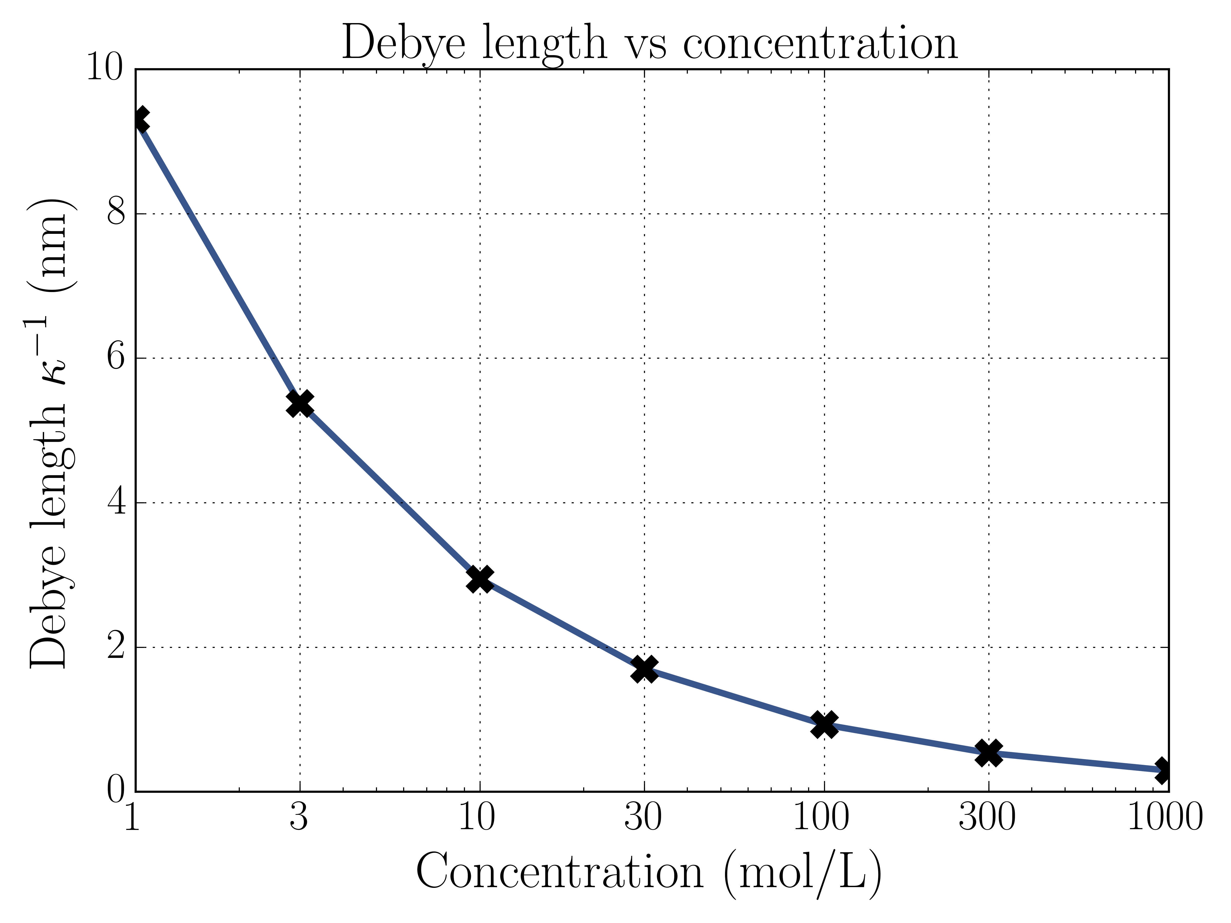
In an experiment we don’t know $\sigma$, and $\psi_{0}$ is usually what’s measured instead. We define the Debye length $\lambda_{D}\equiv\kappa^{-1}$, an important parameter which is the measure of the size of the EDL. Notice that the Debye length does not depend on the surface charge $\sigma$, but does depend on the bulk ion concentration $C_{0}$. This means that highly concentrated ion solutions screen over shorter lengths than diffuse solutions. Here’s a plot of the Debye length for different bulk concentrations.

Plugging the solution for the electrostatic potential back into the Boltzmann equation yields the equations for $C^{\pm}$. With equations in-hand, we can begin to understand the structure of the EDL. Let’s take a look at the most relevant features, the electrostatic potential $\psi$, the number densities of each species $C^{\pm}$, and the difference in number densities of the two species $C^{+}-C^{-}$, which is proportional to the charge density in the solution. We’ll focus on exploring the relationship between these features and the surface charge density, $\sigma$. Note that solving for $\psi$, $C^{+}$, and $C^{-}$ requires knowing the surface potential $\psi_{0}$. This can be done via the Grahame-equation above, but must be solved numerically since it is a transcendental equation for $\psi_{0}$ given $\sigma$. I used the scipy.optimize package to solve the equation. Here’s a plot of the relationship between $\sigma$ and $\phi$ from the Grahame equation:

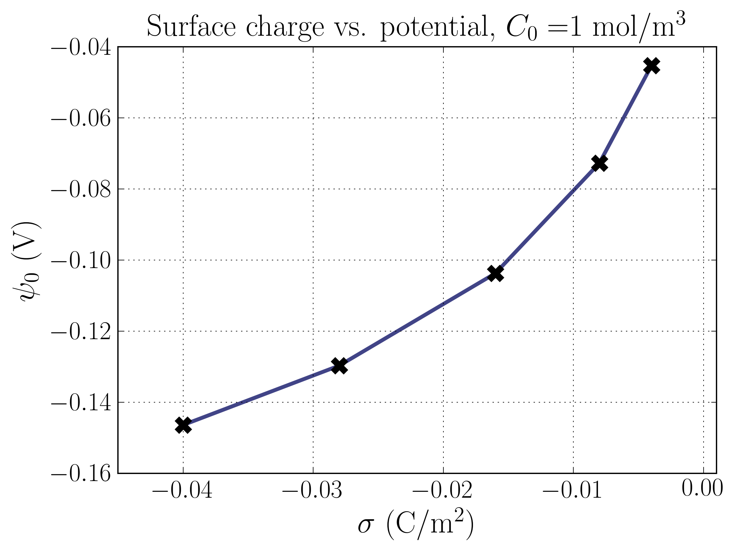
Interestingly, the relationship isn’t perfectly linear as one might naively think. Without the ions (i.e. just a charged plate), the surface potential is directly proportional to the surface charge. Notice that the surface potential is higher when the solution is more dilute; this makes sense, because the same charge is screened over a greater distance, and the electric potential is proportional to the inverse of the distance; because the screening ions are at a greater distance from the surface, they contribute less positive potential.

The following two plots show the electrostatic potential and ion number densities as a function of distance from the charged surface for two different solution concentrations, $C_{0}=1/N$ mol/m$^{3}$, and $C_{0}=100/N$ mol/m$^{3}$.

A couple things to point out. First, note that the surface potential $\psi_{0}$ matches the results given by the Grahame equation above. In both cases there are sharp potential changes in the EDL that taper off away from the surface. This reflects the fact that the electric fields die off in the bulk.

Here are some plots of the ion number densities. The key results here are that the difference in densities, $C^{+}-C^{-}$, which is proportional to the net volume charge can be very large, and that the total ion number density $C^{+}+C^{-}$ can greatly exceed the bulk concentration $C_{0}$.

1 mol/m$^{3}$

100 mol/m$^{3}$

That’s about it for the EDL! In future posts, I’ll get into how the EDL affects transport in nanopores.

comments powered by Disqus